What is the Finite Element Method?

Imagine you are an engineer tasked with designing a new wing for an aircraft. You need to know precisely how it will bend under immense aerodynamic forces, where the stresses will concentrate, and how it will vibrate. Or perhaps you are a medical researcher simulating the flow of blood through an artery, or a civil engineer ensuring a new skyscraper can withstand an earthquake. These problems share a common thread: they involve understanding the complex behavior of a physical system governed by intricate mathematical equations that are impossible to solve by hand.

The tool that makes answering these questions possible is the **Finite Element Method (FEM)**. It is a powerful computational technique for obtaining approximate numerical solutions to the complex differential equations that describe physical phenomena in engineering and mathematical physics. In essence, FEM is a digital simulation toolkit that allows us to break down the impossibly complex into the manageably simple.

The Core Idea: Divide and Conquer

The name itself reveals the method’s fundamental principle. “Finite Element” refers to the practice of subdividing a large, complicated system into a finite number of smaller, simpler pieces, called **elements**. These elements—which can be triangles, quadrilaterals, tetrahedra, or other simple shapes—join together at points called **nodes** to form a mesh, a patchwork quilt that approximates the original geometry.

Think of it like trying to calculate the area of an irregularly shaped lake. Measuring it directly would be difficult. But if you draw a grid over a map of the lake, you can count the number of complete squares inside it, estimate the area of the partial squares on the edge, and sum them all up for a very accurate total. The finer the grid, the more accurate your answer. FEM operates on the same principle of discretization.

This process of meshing transforms a problem with an infinite number of points (a continuous system) into a problem with a finite number of unknowns (a discrete system). This is crucial because while the governing equations of nature are continuous, computers are digital; they excel at solving problems with finite, discrete data.

The Mathematical Engine: How FEM Works

The magic of FEM lies in what it does with each of these small elements. The process can be broken down into a series of steps:

1. Discretization (Meshing): The physical domain (the bridge, the engine part, the femur bone) is divided into a mesh of finite elements. The density of the mesh can be varied; areas where high stress or rapid change is expected, like around a hole or a sharp corner, can have a finer mesh for greater accuracy.

2. Element Formulation: For each element, a simple polynomial function is chosen to approximate the behavior of the unknown quantity we’re solving for (be it displacement, temperature, pressure, etc.) within that element. This method assumes that the solution for the entire complex domain can be well-approximated by stitching together these simple, piecewise functions.

3. Assembly: The equations governing each element are meticulously combined into a much larger system of algebraic equations that model the entire structure. This system embodies the collective behavior of all the elements, respecting how they connect and interact at their shared nodes.

4. Solving: This large system of equations, which can number in the millions for a complex analysis, is solved by the computer to find the value of the primary unknown (e.g., displacement at each node). Modern supercomputers and efficient algorithms make this formidable task feasible.

5. Post-Processing: Finally, with the primary solution known, the software calculates other important derived results, such as stress, strain, heat flux, or fluid velocity. This data is then presented to the engineer through colorful contour plots, animations, and graphs, transforming vast columns of numbers into intuitive visualizations that highlight critical areas like maximum stress or failure points.

 A Brief History and Ubiquitous Applications

While its mathematical foundations were laid by early 20th-century mathematicians, the modern Finite Element Method was pioneered in the 1950s and 1960s by engineers in the aerospace and civil engineering industries. They needed ways to analyze complex structures like airframes and dams, and the advent of the digital computer provided the necessary calculating power. What began as a tool for structural mechanics has since exploded into virtually every field of engineering and science.

• Today, FEM is the backbone of  Computer-Aided Engineering (CAE) software. It is used for:
  * Structural Analysis: Predicting deformation, stress, and vibration.
  * Thermal Analysis: Modeling heat transfer and temperature distributions.
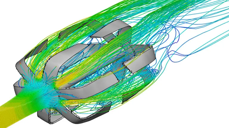
  * Fluid Dynamics: Simulating the flow of liquids and gases (Computational Fluid Dynamics – CFD).
  * Electromagnetics: Analyzing magnetic and electric fields.
  * Biomechanics: Designing prosthetic implants and studying blood flow.

In conclusion, the Finite Element Method is far more than a mere mathematical trick. It is a fundamental paradigm that empowers us to model, simulate, and understand the physical world with unprecedented fidelity. By harnessing the power of discretization and computation, FEM extends the reach of human ingenuity, allowing us to design safer cars, more efficient airplanes, life-saving medical devices, and resilient infrastructure, all within the virtual realm before a single physical prototype is ever built. It is, without exaggeration, one of the most significant engineering advancements of the last century.